Lab 2: Inertial Measurement Unit

• Add the IMU to the robot
• Start running the Artemis and sensors from a battery
• Record a stunt with the RC robot

1. Setup the IMU
2. Accelerometer
3. Gyroscope
4. Sample Data
5. RC Robot Stunt

In order to know that the board is running, I made it so that the Artemis' LED blinks thrice on start-up. This is showcased in the following video:

Video 3: LED blink start-up indication

In order to convert the accelerometer data into pitch and roll, I used the following equations presented in class:

The multiplication by 180 and division by pi, is simply to convert radians into degrees.

The following video showcases the output of the accelerometer for pitch and roll in degrees:

Video 4: Accelerometer Pitch and Roll output in degrees

Based on the previous videos, and other testing conducted during the lab, I concluded that the accelerometer is accurate enough, to the point where a two-point callibration is not necessary. After all, it is known that our robot cars will not have extremely accurate sensor readings in general.

Frequency Spectrum Data Analysis:

The artemis code for data collection and sharing with the computer is the following:

case GET_ACC_DATA:
    
    float accelMicros;
    float theta; //pitch
    float phi; //roll

     accelMicros = 0;
     theta = 0; //pitch
     phi = 0; //roll

    if (!success) {return;}

    // Collection of 2500 data points
    for (int i = 0; i < 2500; i++) { 
    while (!myICM.dataReady()) {}
    myICM.getAGMT();

    accelMicros = micros();
    theta = atan2(myICM.accX(), myICM.accZ()) * 180 / M_PI; 
    phi  = atan2(myICM.accY(), myICM.accZ()) * 180 / M_PI; 
    
    timestamps[i] = accelMicros;
    thetas[i] = theta;
    phis[i] = phi;
}

// send one message to computer for each index of the data arrays
for (int j = 0; j < 2500; j++) { 
    tx_estring_value.clear();
    tx_estring_value.append("T:");
    tx_estring_value.append(timestamps[j]);
    tx_estring_value.append(",P:");
    tx_estring_value.append(thetas[j]);
    tx_estring_value.append(",R:");
    tx_estring_value.append(phis[j]);
    tx_characteristic_string.writeValue(tx_estring_value.c_str());
}
            break;

The previous code sends 2500 data points to the computer where each data point contains Time, Pitch and Roll. Then, the computer receives it through the following python handler function which also saves it to the computer as a CSV file.

def accelerometer_handler(uuid, byteArray):
    string = ble.bytearray_to_string(byteArray).strip()
    t, p, r = string.split(",")
    time = float(t[2:])  
    pitch = float(p[2:])   
    roll = float(r[2:])  
    #print(f"{time_value},{pitch},{roll}\n")
    with open("accelerometer_data.csv", "a+") as file:
        file.seek(0)
        if file.read(1) == "":
            file.write("Time,Pitch,Roll\n")
        file.write(f"{time},{pitch},{roll}\n")

The data isn't as noisy as I had expected. Our IMU has a "built-in" low pass filter. However, in the future, the IMU is going to be inside the robot's body right next to the motors. This, in addition to the fact that there are probably going to be other sources of noise, suggested I should implement a low-pass filter.

Examining my original data, I saw that the "real" data were under 5 Hz above which there was noise.

My total sampling time was 7020988 microseconds = 7.020988 seconds and I took 2500 samples. This means my Sampling Rate was 356Hz or Sampling Period of ~0.0028 s. For a low-pass filter with a cut-off frequency of 5 Hz, RC = 1/(2π5) = ~0.0318 s. From these, we can derive α = 0.0028/(0.0028+0.0318) = ~0.081

The following 4 plots are with me hitting the lab counter (a bit unsuccessfully I would add as I barely managed to make the IMU viberate). Note that the pitch in the Time Domain is negative because of how I had left the IMU to rest on the counter. You can see this in Video 3.

These plots show the unfiltered (raw) and filtered (with the 5Hz cutoff Low-pass filter) data, both in the time and frequency domain.

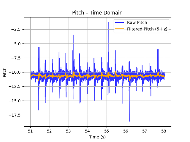
Figure 1: Pitch Time Domain

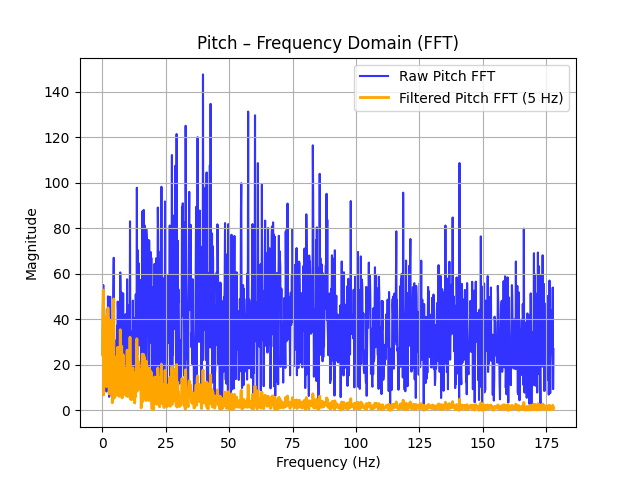
Figure 2: Pitch Frequency Domain

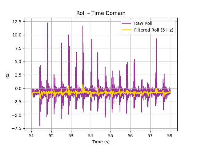
Figure 3: Roll Time Domain

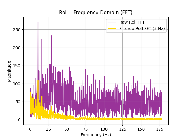
Figure 4: Roll Frequency Domain

The following figures is when I was moving the IMU with my hand:

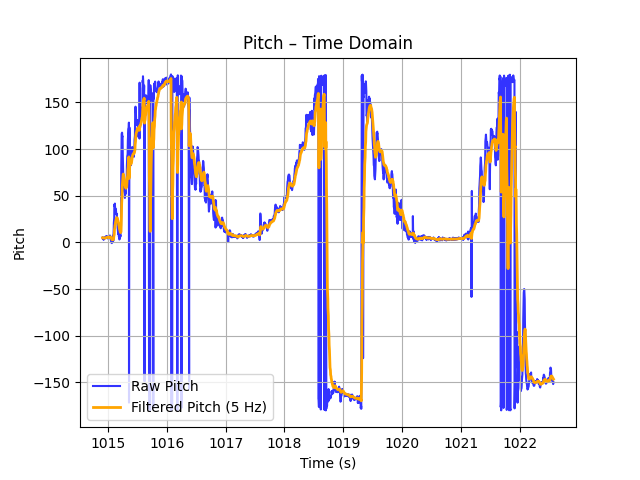
Figure 5: Pitch Time Domain while moving IMU

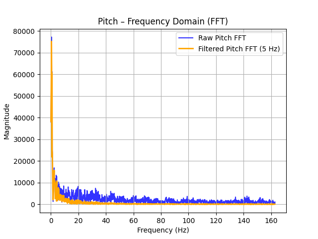
Figure 6: Pitch Frequency Domain while moving IMU

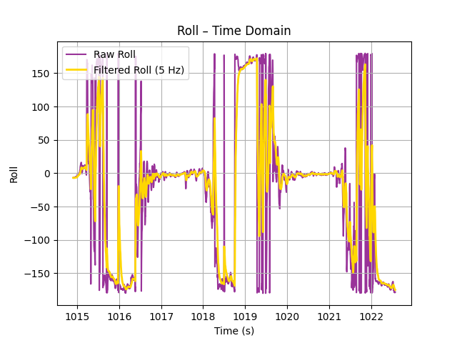
Figure 7: Roll Time Domain while moving IMU

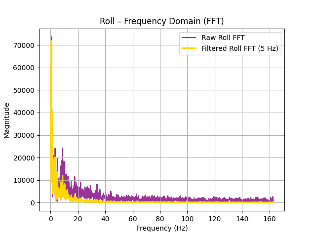
Figure 8: Roll Frequency Domain while moving IMU

Though there is still some noise present after implementing the low-pass filter, the output of the lp filter was vastly improved compared to the raw data.

In order to convert the gyroscope data into pitch and roll, I used the following equations presented in class:

With these equations I got the following results:

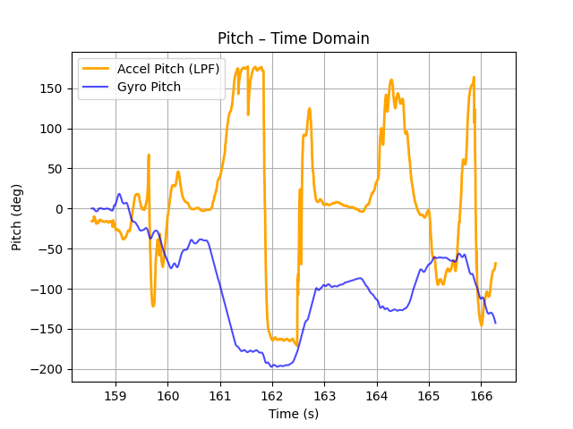
Figure 9: Pitch Time Domain

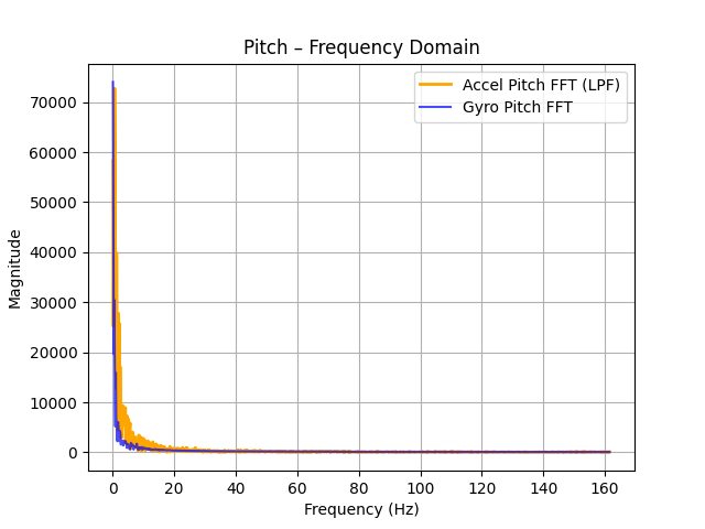
Figure 10: Pitch Frequency Domain

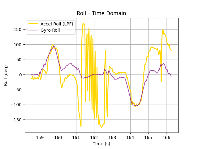
Figure 11: Roll Time Domain

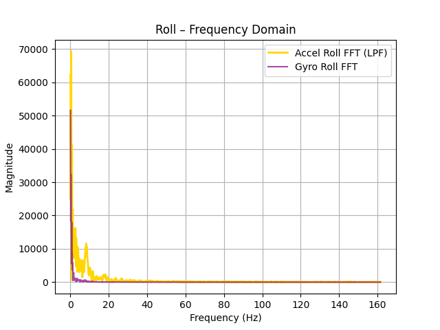
Figure 12: Roll Frequency Domain

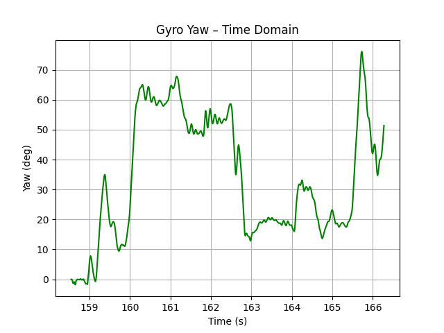
Figure 13: Yaw Time Domain

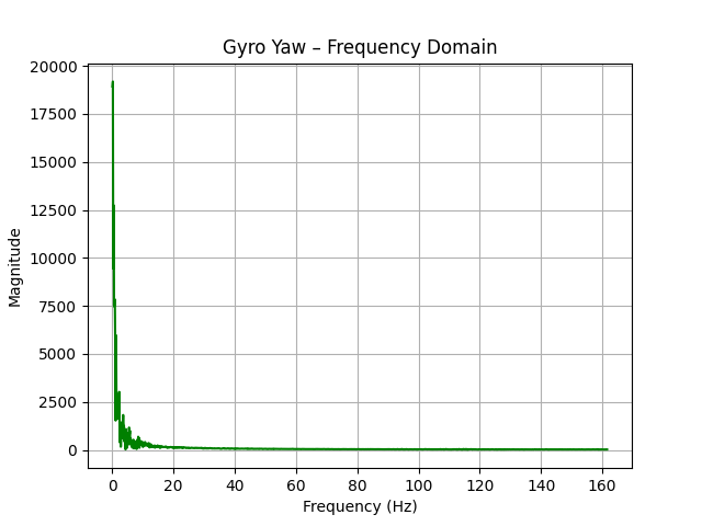
Figure 14: Yaw Frequency Domain

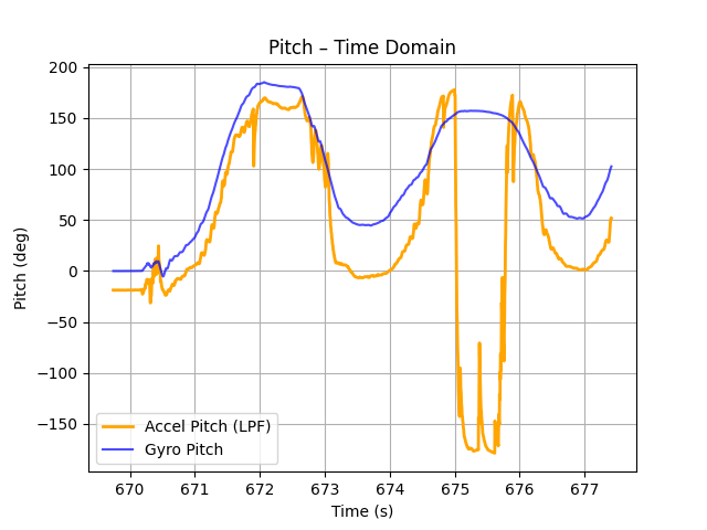
Figure 15: Pitch Time Domain (corrected)

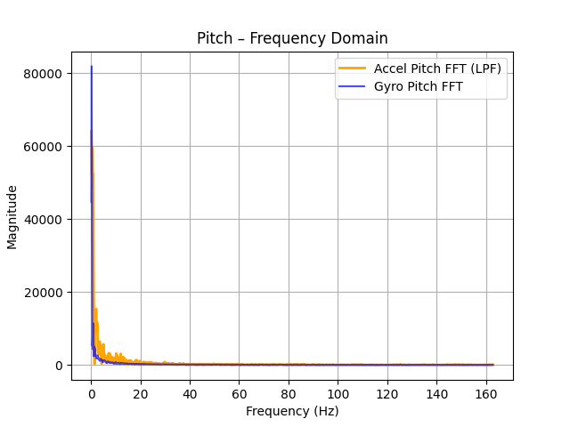
Figure 16: Pitch Frequency Domain (corrected)

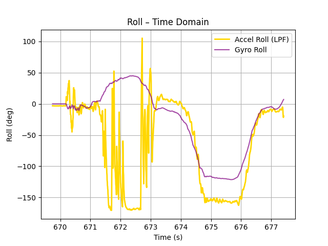
Figure 17: Roll Time Domain (corrected)

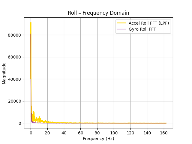
Figure 18: Roll Frequency Domain (corrected)

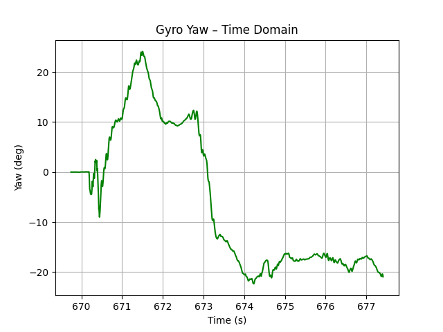
Figure 19: Yaw Time Domain (corrected)

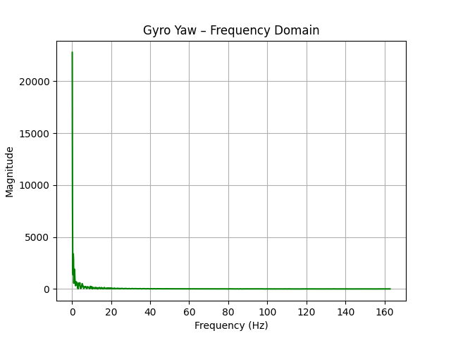
Figure 20: Yaw Frequency Domain (corrected)

The two following figures are without and with 4ms delay respectively. Our original sampling rate was ~2000 microseconds. 4 millisecond delay ==> 4000 microsecond delay ==> 6000 microseconds total sampling time ==> tripling the sampling time. The results from the following figures show that adding a delay has an effect on the amount of drift present. We can observe that for the same amount of time that has passed, more drift has been introduced:

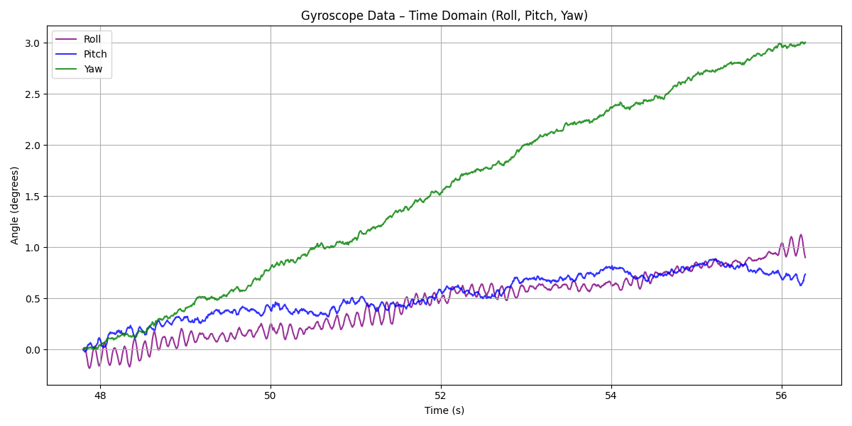
Figure 21: No delay

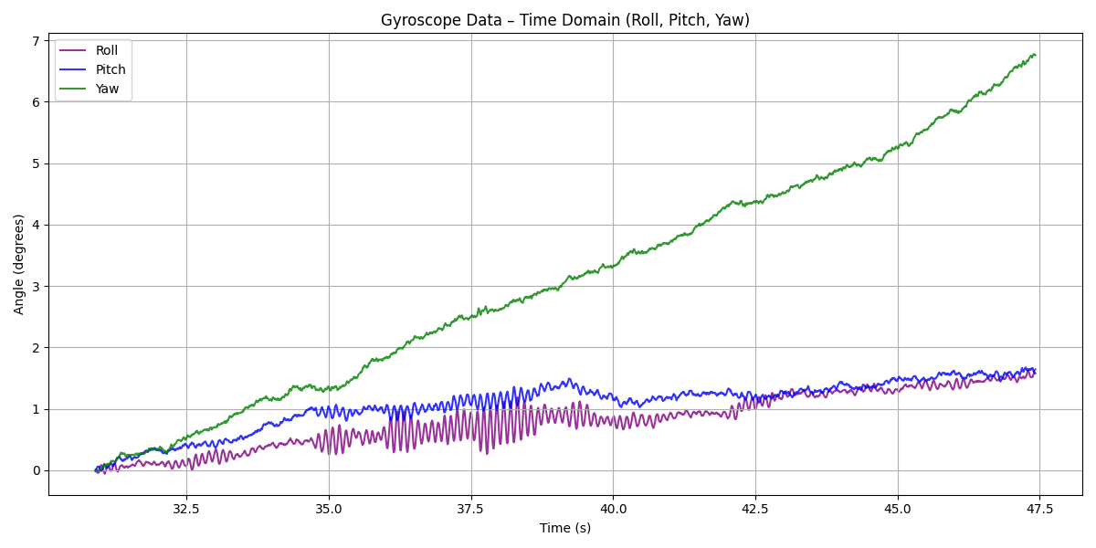
Figure 22: 4 ms delay

Complementary Filter:

From the following plots with alpha=5% and alpha=10% respectively, we can see that the difference is miniscule but a=5% produces a slightly better result.

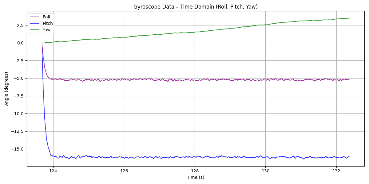
Figure 23: alpha = 5%

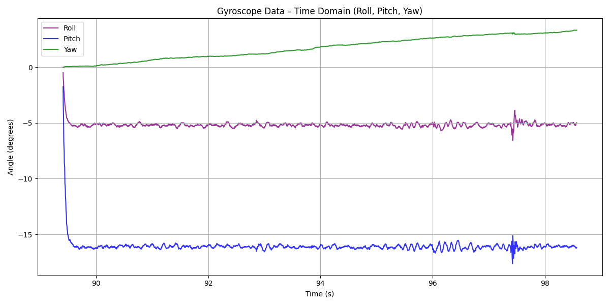
Figure 24: alpha = 10%

Finally, here we can see the range and accuracy of the complementary filter with a=5%. Note that I was holding it without keeping my hand stable which produced quick vibrations. We can also observe that the drift here is negligible.

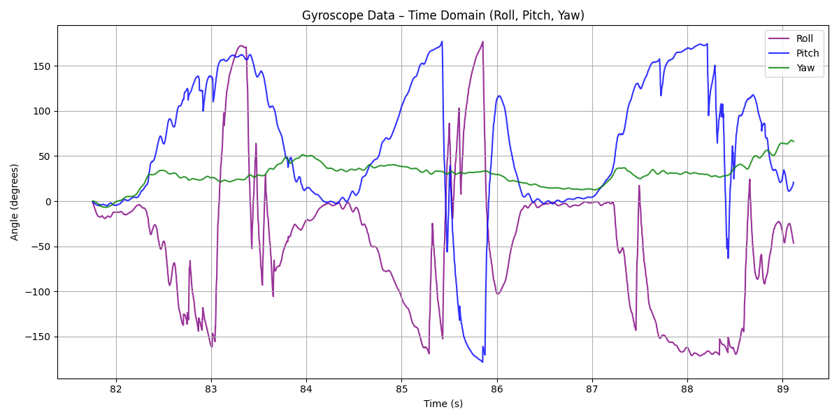
Figure 25: working range, accuracy lack of susceptibility to drift or quick vibrations

Sampling Data Points via the loop is slightly slower at 3554 microseconds per data point, while before, with the same complementary filter, it was 3470 microseconds. This is equivalent to ~281.4 measurements per second.

void loop(){
    // Listen for connections
    BLEDevice central = BLE.central();

    // If a central is connected to the peripheral
    if (central) {
        Serial.print("Connected to: ");
        Serial.println(central.address());

        // While central is connected
        while (central.connected()) {
            // Send data
            write_data();

            // Read data
            read_data();

if( collecting_data && (data_points < 2500)){
  loop_iterations++;
  
  if(myICM.dataReady()){

  myICM.getAGMT();
        Now = micros();
        dT = (Now - T0) / 1000000.0;
        T0 = Now;

        // Accelerometer angles
        Acc_pitch = atan2(myICM.accX(), myICM.accZ()) * 180.0 / M_PI; 
        Acc_roll = atan2(myICM.accY(), myICM.accZ()) * 180.0 / M_PI; 

        float Gyro_increment_pitch = -myICM.gyrY() * dT;  // minus needed
        float Gyro_increment_roll = myICM.gyrX() * dT;   // minus not needed
        
        Comp_pitch = (1.0 - alphaCont) * (Comp_pitch + Gyro_increment_pitch) + alphaCont * Acc_pitch;
        Comp_roll = (1.0 - alphaCont) * (Comp_roll + Gyro_increment_roll) + alphaCont * Acc_roll;
        
        // Yaw: gyro only
        Gyro_yaw += myICM.gyrZ() * dT;

        timestamps[data_points] = Now;
        pitchs[data_points] = Comp_pitch;
        rolls[data_points] = Comp_roll;
        yaws[data_points] = Gyro_yaw;

  data_points++;
}}}
        Serial.println("Disconnected");
}}

and these as my flag setter commands for the Artemis:

case START_COLLECTING_DATA:
    data_points = 0;
    loop_iterations =0;
    T0=micros();
    Gyro_yaw = 0;
    

   collecting_data = true;
   break;

case STOP_COLLECTING_DATA:
   collecting_data = false;
    for (int j = 0; j < data_points; j++) { 
        tx_estring_value.clear();
        tx_estring_value.append("T:");
        tx_estring_value.append(timestamps[j]);
        tx_estring_value.append(",P:");
        tx_estring_value.append(pitchs[j]);
        tx_estring_value.append(",R:");
        tx_estring_value.append(rolls[j]);
        tx_estring_value.append(",Y:");
        tx_estring_value.append(yaws[j]);
        tx_characteristic_string.writeValue(tx_estring_value.c_str());
    }   
    Serial.print("Completed Loop Iterations: ");
    Serial.print(loop_iterations);
    Serial.print(" and Collected Data Points: ");
    Serial.println(data_points);
   break;

My car's name is Zeus. No, I did not name it myself. It is pronounced Zefs, just like Odyssefs.

After experiencing the car, I can tell it slips a lot, it is very unstable and it doesn't turn well. Also it can flip when stopping after going fast in a line. I believe the turning aspect will be much better after Zeus has successfully transisioned into a proper robot.

Video 5: RC Robot 1st Stunt

Video 6: RC Robot 2nd Stunt

Lab 2 successfully integrated the IMU to the Artemis and utilized the accelerometer and gyroscope it has to collect and send data to the computer. The data acquisition is set up to send data points to the computer and ready for extension in subsequent labs.

What challenged me the most was the lack of time to do everything sufficiently.

I really like the way I have made the Artemis print the loop iterations and collected data points to see whether the loop runs faster than the IMU readies data.